Disclaimer

This article was drafted with the help of Copilot (AI) – so if it is unusually well structured or my English sounds unusually polished, that’s probably why 😊. I’m not a DAX expert (yet), and the DAX code used here was generated by Copilot too. It worked well for testing, but I’d recommend reviewing it thoroughly before using it in production.

The test reflects my specific use case – a many-to-many relationship between a fact and a dimension table. Your scenario might differ, so results may vary.

Feedback from experienced Power BI developers is always welcome!

Foreword

After more than a decade in Business Intelligence and two years of working with Power BI, I’ve come to appreciate how different the Tabular Model behaves compared to SQL Server or SSAS Multidimensional. This post documents my deep dive into modeling many-to-many relationships between fact and dimension tables – not just between dimensions, as often discussed.

As part of my learning journey, I watched Different types of many-to-many relationships in Power BI by Marco Russo. However, the video focuses on relationships between dimensions, while my challenge lies in modeling a many-to-many relationship between a fact table and a dimension.

If you’re short on time, feel free to jump straight to the Results for the key takeaways.

Starting Point

My existing SSAS Multidimensional solution loads in 1–2 seconds. The new Power BI model with SSAS Tabular takes 3–5 seconds – noticeably slower. That got me curious: is it the technology, the modeling, or something else?

I’ve always modeled this scenario using a bridge table to handle many-to-many relationships. But Power BI is different, so I decided to test several modeling variants to compare performance, model size, and maintainability.

The Business Requirement

The data is from a rule-based engine:

• A new transaction comes in.
• 0–n rules may trigger.
• A total score is calculated.
• If the score exceeds a threshold a team investigates.

Each case can be queried multiple times over time.
In Power BI we would like to track:

• Transactions: each and every query
• New Transactions: first query per case.
• Recent Assessments: latest query per case.

Rules are grouped into categories, and multiple rules can trigger per transaction. This makes the metric semi-additive – a classic BI challenge. Here’s an example:

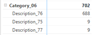
Let’s take a quick look at Rule Category 6:

• Triggered Rules: 76, 75, and 77
• Requests: 702
• Rule Hits: 688 + 9 + 9 = 706

What does that tell us?

• At least one request triggered multiple rules from the same category.
• The total rule hits exceed the number of requests – a textbook case of a semi-additive metric.
• This is exactly why modeling and aggregating correctly matters – especially when slicing by category.

Test Data

To keep things manageable but realistic I took a sample from the original dataset:

Metric	Original Dataset	Test Subset
Transactions	15,000K	1,000K
Rule Hits	62,000K	3,500K
Rule Combinations	593K	167K
Hits per Transaction	4.2	3.5
Number of Rules	276	271

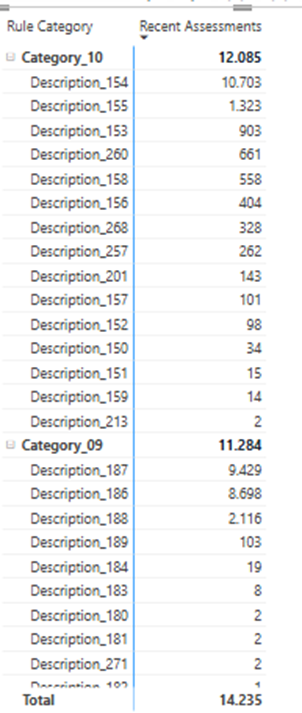
Query 1: Recent Assessments by Rule Category

This query evaluates the number of recent assessments per rule category within a specific date range. I chose the last month 07.07.25-06.08.25 for testing. The result is semi-additive as explained before. It’s a good stress test for model structure and DAX logic.

Query 2: Top Rules

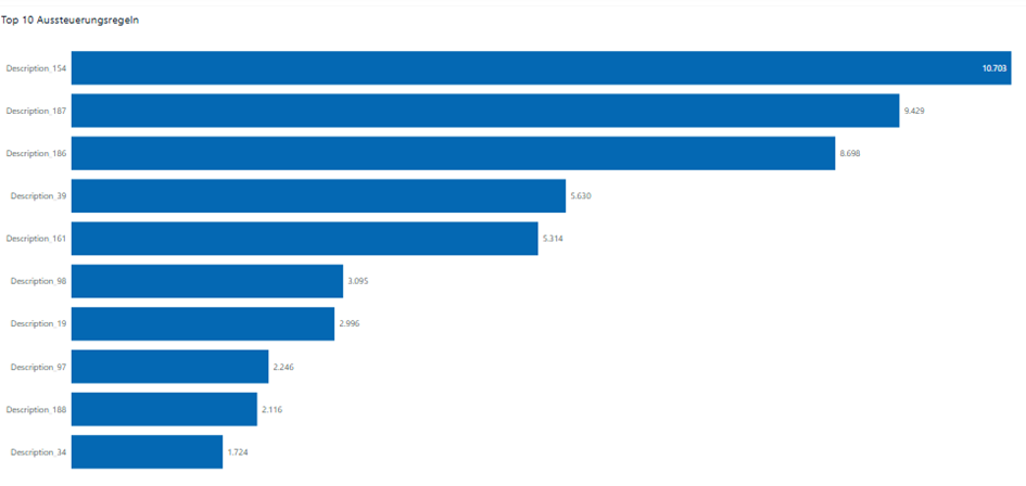
This query identifies the most frequently triggered rules within the same date range. It’s a straightforward ranking based on the number of rule hits, grouped by rule description and sorted descending.

It’s less complex than Query 1 but still benefits from efficient model design and indexing – especially when working with millions of rows and many-to-many relationships.

Test Methodology

To ensure consistent and reliable performance measurements, I followed the approach described by Nikola Ilic:

• Used DAX Studio to run all queries.
• Enabled Server Timings and Query Plan.
• Cleared the cache before each run.
• Measured runtime in milliseconds, broken down into:
  • Formula Engine (FE) time
  • Storage Engine (SE) time

Each query was executed three times, and the last result was used for comparison.

Test Results

I tested six different modeling approaches. You can read about them in the Appendix. Here’s the summary ordered by query performance:

Approach	Granularity	Relationship	PBIX Size (MB)	# Tables for Join	Query 1 Summary	Query 2 Summary
1. Fact High Granularity (prebaked)	1 row per rule & transaction	N:1	49.5	1	23 ms (48% SE)	17 ms (59% SE)
2. Fact High Granularity (DAX Magic)	1 row per rule & transaction	N:1	51.1	1	173 ms (49% SE)	17 ms (71% SE)
3. Fact 1nn1 Cardinality	1 row per transaction	1:N, N:1	62.6	2	338 ms (97% SE)	311 ms (95% SE)
4. FactDimension 1nn1 Cardinality	1 row per transaction	1:1, 1:N, N:1	62.6	3	422 ms (96% SE)	455 ms (96% SE)
5. Matrix 1nn1 Cardinality	1 row per transaction	N:1, 1:N, N:1	46.7	3	648 ms (99% SE)	654 ms (99% SE)
6. Matrix MN Cardinality	1 row per transaction	M:N, N:1	40.8	2	1263 ms (99% SE)	627 ms (99% SE)

Resources

I’m making all test model variants—including the PBIX files and associated queries—available for download. This gives you full transparency into the setup and lets you explore performance differences hands-on.

👉 Download: PBIX Test Models

Key Observations

• The prebaked high granularity model was shockingly fast – 7x faster than the next best in Query 1.
• Models with shorter join paths to the Rule table performed better.
• My previous go-to – the Matrix dimension model – landed second to last. Time to rethink that one.
• The M:N cardinality model was the slowest, despite having the smallest PBIX file size.

Conclusion

This test was eye-opening. I learned that:

• High granularity fact tables (one row per rule hit) perform best in Power BI in my use case. They eliminate the need for many-to-many relationships to dimension tables.
• Prebaking aggregations can significantly boost performance – even if it feels “old school.”
• The modeling approach matters more than I expected. What worked in SSAS Multidimensional doesn’t always translate well to Tabular.

Next Steps

• Rebuild the fact table with high granularity.
• Explore DAX optimizations to speed up the “DAX Magic” variant. Feedback is highly appreciated 😉.
• Run tests on the full dataset.

Appendix: Modeling Variants in Detail

Here’s a quick walkthrough of the six modeling approaches I tested – each with its own quirks and trade-offs.

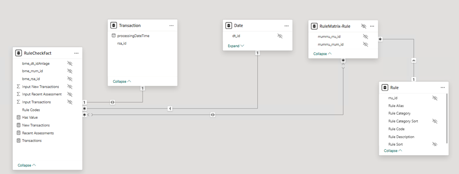
Matrix 1nn1 Cardinality

Granularity: 1 row per transaction

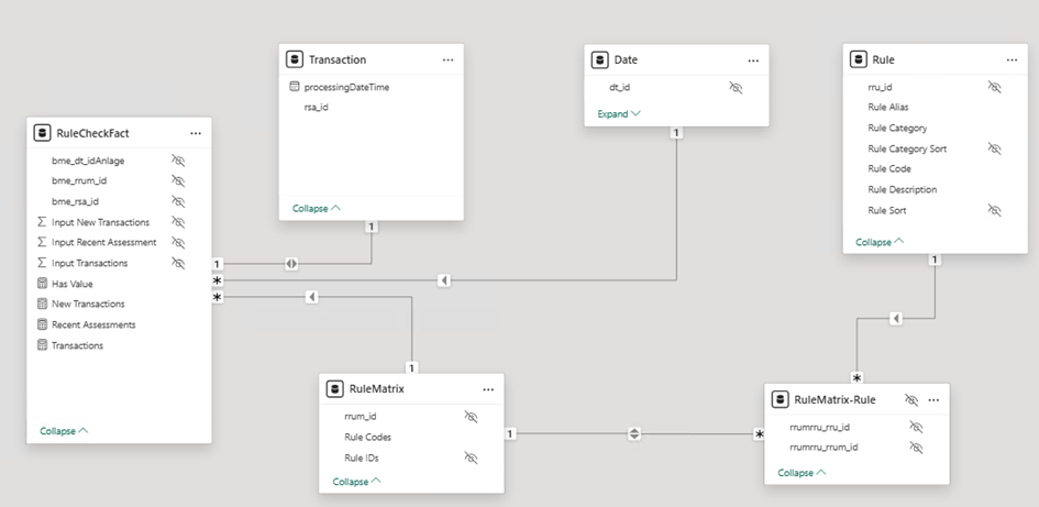
• Based on my original SSAS Multidimensional model.
• Uses a RuleMatrix dimension with all rule combinations (167K rows in test).
• Bridge-Table connects RuleMatrix to Rule.
• Requires bidirectional filtering, which is necessary to propagate filters from the Rule dimension down to the fact table. Yes, I am aware of the potential risks 😉.
• Relationship path: Rule → RuleMatrix → RuleMatrix-Rule → Fact
• I originally learned this technique from the book The Microsoft Data Warehouse Toolkit by Joy Mundy and Warren Thornthwaite – still a great resource for dimensional modeling fundamentals.
• This setup felt familiar but turned out to be one of the slower options.

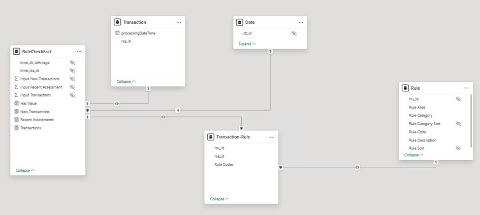
Matrix MN Cardinality

Granularity: 1 row per transaction

• Similar to above but skips the RuleMatrix dimension.
• Direct M:N relationship between Fact and Bridge table.
• Rule codes stored directly in the fact table.
• Also requires bidirectional filtering for filter propagation from Rule to Fact.
• Surprisingly, this was the slowest model in the test – despite having the smallest PBIX file.

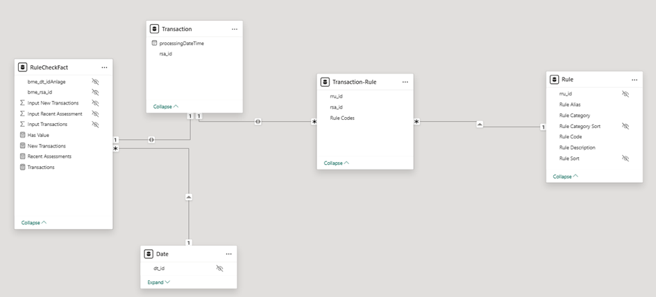
Fact 1nn1 Cardinality

Granularity: 1 row per transaction

• No matrix involved.
• Bridge table contains one row per transaction and rule hit (4.2M rows in test).
• Straightforward 1:N relationship to Rule.
• Performs better than the matrix variants, but still not ideal.

FactDimension 1nn1 Cardinality

Granularity: 1 row per transaction

• Similar to the previous, but the bridge connects to a fact dimension instead of the main fact table.
• Adds complexity without clear performance benefits.
• Slightly slower than the direct fact variant.

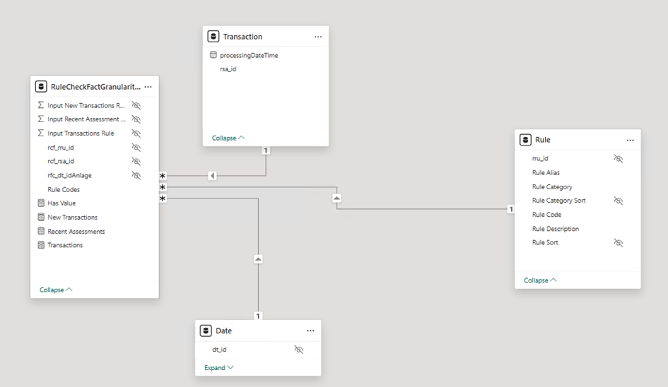
Fact High Granularity (Prebaked)

Granularity: 1 row per transaction and rule

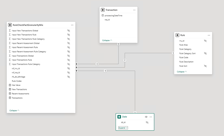
• Fact table contains one row per transaction and rule.
  • This feels a bit odd to me: The data doesn’t naturally live at that granularity level as it is measured per transaction.
• Aggregations (per rule, category, and global) are precalculated in the source system.
• Measures dynamically switch between input columns depending on the filter context.
• This technique feels a bit “old school” – I first learned it over 13 years ago, during my early career working with SQL Server 2008 R2 Analysis Services Standard Edition, where semi-additive measures had to be handled manually due to limited feature support.
• It still works surprisingly well, but comes with trade-offs:
  • Requires more effort in data preparation.
  • Measures must be manually adjusted if new columns or hierarchy levels are added to the Rule table.
  • Less flexible and harder to maintain in dynamic environments.
• Despite that, this variant turned out to be the fastest in my performance tests – especially for Query

DAX Logic

Recent Assessments :=
// DAX Code generated by Copilot...not production-ready
VAR isRuleCategoryFiltered =
    ISFILTERED ( 'Rule'[Rule Category] )
VAR isRuleDescriptionFiltered =
    ISFILTERED ( 'Rule'[Rule Description] )
RETURN
    SWITCH (
        TRUE (),
        // Level Rule: Show Input Measure for Rule
        isRuleCategoryFiltered
            && NOT isRuleDescriptionFiltered, SUM ( 'RuleCheckFactGranularityMix'[Input Recent Assessment Rule Category] ),
        // Level Rule Category: Show Input Measure for Rule Category
        isRuleDescriptionFiltered, SUM ( 'RuleCheckFactGranularityMix'[Input Recent Assessment Rule] ),
        // Level ALL: Show Input Measure for Global
        NOT isRuleCategoryFiltered && NOT isRuleDescriptionFiltered, SUM ( 'RuleCheckFactGranularityMix'[Input Recent Assessment Global] ),
        BLANK ()
    )

Fact High Granularity (DAX Magic)

Granularity: 1 row per transaction and rule

• Same granularity as before, but no pre-aggregated columns.
• All logic handled via DAX using GROUPBY and MAXX.
• Slightly slower than the prebaked version in Query 1, but equally fast in Query 2.
• More flexible, easier to maintain, and better suited for dynamic models.

 DAX Logic

Recent Assessments =
// Measure generated by Copilot...probably not production ready
VAR isRuleCategoryFiltered =
    ISFILTERED ( 'Rule'[Rule Category] )
VAR isRuleDescriptionFiltered =
    ISFILTERED ( 'Rule'[Rule Description] )
RETURN
    SWITCH (
        TRUE (),
        // Level Rule: Sum Input Measure
        isRuleDescriptionFiltered, SUM ( 'RuleCheckFactGranularityRule'[Input Recent Assessment Rule] ),
        // Level Rule Category: Calculate Value per Transaction and Rule Category
        isRuleCategoryFiltered
            && NOT isRuleDescriptionFiltered,
            SUMX (
                GROUPBY (
                    'RuleCheckFactGranularityRule',
                    'RuleCheckFactGranularityRule'[rcf_rsa_id],
                    'Rule'[Rule Category],
                    "AssessmentSum",
                        MAXX (
                            CURRENTGROUP (),
                            'RuleCheckFactGranularityRule'[Input Recent Assessment Rule]
                        )
                ),
                [AssessmentSum]
            ),
        // Level ALL: Calculate Value per Transaction
        NOT isRuleCategoryFiltered && NOT isRuleDescriptionFiltered,
            SUMX (
                GROUPBY (
                    'RuleCheckFactGranularityRule',
                    'RuleCheckFactGranularityRule'[rcf_rsa_id],
                    "AssessmentSum",
                        MAXX (
                            CURRENTGROUP (),
                            'RuleCheckFactGranularityRule'[Input Recent Assessment Rule]
                        )
                ),
                [AssessmentSum]
            ),
        BLANK ()
    )

Additional Modeling Ideas

• Fact Table Design
  • Considered splitting into two fact tables:
    • One at transaction level
    • One at transaction-rule level
  • Dropped the idea:
    • Metrics are the same across both
    • No analytical benefit
    • Current model has few measures
    • All measures must work across all dimensions
• Filter Propagation
  • Using bidirectional filtering between fact and dimension
    • Helps with filter flow
    • Brings ambiguity risks
    • Confident no further relationships will be added
    • Still unsure if this usage is safe due to limited experience
  • Thought about using TREATAS in measures
    • Avoids bidirectional relationships
    • More robust in complex models
    • But: all measures rely on Rule relationships
    • Applying TREATAS everywhere feels impractical

Final Words

This was my first deep modeling test in Power BI. I welcome feedback from fellow BI professionals – especially those with more DAX and modeling experience. Sometimes, challenging your own assumptions leads to the biggest breakthroughs.