I already did a quite extensive write-up on some sessions from Conference Day 2 at PASS Summit 2019.

• Cybersecurity is everyone’s problem: An extract from the Keynote of Day 2 at Pass Summit
• Survival Techniques for the lone DBA (Pass Summit 2019 Conference Day 2)
• Successfully communicating with your customers (Pass Summit 2019: Conference Day 2)

Here I would like to share the remaining sessions I went to.

Design Strategies and Advanced Data Visualization

This was quite an interesting session by James McGillivray on report design. The session had a lot of demos in Power BI nevertheless this is a topic which can be applied to every reporting tool.

He first spoke a bit about Design Theory which is a new concept to me. If you happen to be in the same spot check out his write up here. Design Theory basically consists of the following six elements:

• Balance
• Proximity
• Alignment
• Repetition
• Contrast
• Space

One important thing James mentioned is that this technique works best if we know what the user is gonna look at respectively we have a mostly static report. If the report is highly configurable by the end user and can therefore change it becomes more challenging to apply design theory principles.

The next topic covered were best practices. The big headline here would be simplicity to me: Keep charts simple (that’s very well related to the IBCS standard and what Hichert proposes), do things consistently across multiple reports and spend as much real estate for data (also known as Data/Ink-Ratio or Signal/Noise-Ration and something which Nicolas Bissantz promoted as well leveraging sparklines.

Color is also quite important relating to reporting and James showed us different ways to do color…with the additional things to be aware of.
There are mainly three types of color schemes:

• monochromatic: where you take on colour and do shading from light to dark
• analogous: where you take three colours which are next to each other on the color wheel
• complimentary: where you take one color and the exact opposite color on the color wheel (opening up the possibility to do quite strong highlighting)

Next was Grid theory, which is nowadays most prevalent with modern reporting applications like PowerBI. If you arrange your visuals into a tabular format this results in a very clean layout that is pleasing to the eye. You should pay attention of introducing gutters as well meaning that you have some space in between your visuals in order to have them better to be distinguished.

The great session concluded with a presentation of accessibility and the argument that accessibility is good for everyone….not only disabled people. As an example James mentioned cut-down-curbs introduced for making live easier for wheelchair users. It turned out that after the change a lot of more people did take advantage from that like parents with strollers, cyclists and so on. James recommended Meagon Longoria’s checklist for accessiblity especially within Power BI. He also showed an impressive demo on how using alt texts and tab order could help a blind person in accessing the report using Windows Narrator.

From Adaptive to Intelligent Query Processing

For the last session of the day I chose Hugo Kornelis talking about Intelligence Query Processing. Microsoft has already introduced a number of Query Optimization Features with SQL Server 2017 called “Adaptive Query Processing”. With SQL Server 2019 this feature set is enriched further and also made available to rowstore indexes. First of all I was quite impressed by Hugo running his demos on SQL Server 2019 RTM which was just released one day before. We all crossed fingers regarding the outcome and there were no issues.

The classic problem with estimated plans

If a query is fired off to SQL Server it basically goes through two stages: Optimization and Execution.

Within the optimization phase SQL Server builds the execution plan. The execution plan mainly relies on information from statistics applied to calculating an estimate how many rows will come back per operator.

Then the query goes into execution. Hugo paraphrased it nicely by stating that it is just as in most big companies…between the “department” of query optimization and query execution there is one big wall. If the plan is run and the engine realizes, that it turns out to be not optimal (like estimated 10 rows and actually received 10.000 rows) there is no way of getting it back to the optimizer and tell it about it.

This is a classic problem which typically led to a degradation in performance. A typical example is a select from a table with skewed data. For one id queried the query might return just a handful of rows and it is best to use a nested loop join. However if the query is rerun the same plan could be used (I write “could” here because I am aware that there are a number of special situations where you could shout out to me and say “You are incorrect about that”…but that’s how it works in most cases).However, having the query now returning 10.000 rows the nested loop join operator gets incredibly slow as it doesn’t scale well with growing number of values. Typically one way or the other (nested loop first or hash match first) you hit situations where the plan being executed is just terribly inefficient.

Adaptive Joins

The address this problem, Microsoft introduced the Adaptive-Join-Operator  in SQL Server 2017 but only for columnstore indexes. With SQL Server 2019 we can get batch mode on rowstore indexes as well and therefore the adaptive join is now applicable to a wider range of uses cases.
I know, I am short on content her guys…I went through the process of describing join types and trying to bring this to you. However I realized that this very much resembles boiling the ocean and there are already great other resources out in the Internet. For further reference please take a look at the following blogs:

• Adaptive Joins in SQL 2019 and Parameter Sniffing (Brent Ozar)
• Adaptive Join as an Operator (Hugo Kornelis)
• Anatomy of an Adaptive Join (Erik Darling)

Interleaved Execution

If you happen to use a Multi-Statement-Table-Valued-Function (aka MSTVF) performance typically is not great. Why is that? Because in optimization SQL Server had no way of determining how many rows this construct will bring back. Remember optimization and execution being separate processes with a wall in between? Microsoft gave us an estimate of 1 row until SQL Server 2016. Not surprisingly most MSTVFs happened to return more than one row….and once again if you are in the thousands of rows then performance gonna hurt as a nested loop join operator is used instead of a hash match. So with SQL Server 2016 Microsoft started to acknowledge that there are performance issues in regard to MSTVFs and rose the estimate to 100 rows. Well fair enough 100 rows sound a bit more realistic than 1 row however it is still a wild guess and your problems stay the same if happened to have thousands of rows returned.

Therefore with SQL Server 2017 a better way dealing with table variables was introduced. If the query optimizer happens to detect a table variable it pauses the optimization for a short time, populates the table variable and then works with the statistics it gets on the pre-filled table variable.

Problem solved? Well, kind of…Hugo pointed out that the first execution of the table variable is cached. If you now happen to have skewed data and wildly different number of rows per execution than running with the plan first cached might not work out that great. That is a similar issue like the one we are used to with stored procedures and parameter sniffing and of course there are ways to deal with it…one of the easiest just to slam an OPTION (RECOMPILE) at the query. Just be aware of that OPTION(RECOMPILE) respectively generating a new plan on each use leads to a little bit more CPU usage and possibly plan cache bloat.

The next thing to be aware of is that according to Hugo this feature of interleaved execution only kicks in in a very limited amount of cases. However I still think it is useful because (if in effect) it can save you from code rewrites and give you better query performance.

Also have a look at:

• Interleaved Execution (Erik Darling)
• Interleaved Execution in SQL Server 2019 (Wayne Sheffield, comparison between SQL Server 2017 and 2019)

Memory Grant Feedback

Inaccurate estimates also lead to a different problem: Spilling in tempdb. What does that mean?

Before the query runs every operator (e.g. a hash match join) is assigned some workspace in RAM. The space reserved is based on the approximate size of the data being processed and (surprise) the number of rows. You can imagine if the number of rows do not resemble the actual number of rows returned during execution, then we can run into a problem (too little memory reserved). On the other hand reserving too much memory could also pose a problem because of concurrency. On a database server our query is typically not the only query which runs at one point in time. If it would take more memory than needed, the query itself would have no issue but there would be less memory available for other queries due to the over-estimation. In the end if we have too little memory SQL server has to get the remaining memory needed from tempdb. Since tempdb is stored on a disk drive, it typically takes much longer to access it than the RAM directly (I am not that sure about that new Intel Optane Persistent Memory drives though…but hey there’s currently probably just a minority of lucky guys running them anyway).

So what happens now with Memory Grant Feedback? SQL Server is able to adjust the amount of memory used based on the prior execution of one query.
For example if a query runs the first time, gets 15 MB of memory assigned but needs 150 MB, SQL Server will correct the memory grant for the operator in the plan cache and assign more memory the next time the query runs . The exact amount of memory assigned is the actual memory used with an additional safety margin (because our data only ever grows but never shrinks, right?).

This also works the other way around. If we have a query which is assigned way more much memory than it actually needs at execution time, the memory grant is cut down by SQL Server for the next execution. So SQL Server basically tries to get smarter every time we execute a query to save us spills to tempdb. Is this a remedy for every situation? Unfortunately not. Hugo gave the example of a parameterized query based on skewed data. If you happen to run the first execution with a decent number of rows returned (e.g. 10K rows) and run the second execution with only a handful of rows (e.g. 50), then Memory Grant Feedback will most likely kick in and reduce your memory grant. However that gets a problem if you have a high number of rows in the next execution as SQL Server would take the reduced memory grant and start spilling to disk.

Memory Grant has been around since SQL Server 2017 for ColumnStore and is extended to RowStore in SQL Server 2019.

Once again, there already have been some other bright people out there writing about Memory Grant Feedback more in-depth:

• SQL Server 2019 Memory Grant Feedback (Eduardo Pivaral)
• Row Mode Memory Grant Feedback (Rajendra Gupta)
• What’s new in SQL Server 2019: Adaptive Memory Grants (Brent Ozar)

Table-Variable Deferred Compilation

There is an old saying about table variables in SQL Server:

If you think about using a table variable, think again and go for a temp table.

Why is that so? Because table variables at maximum can have a primary key but no additional indexes or statistics.
Therefore you typically get an estimate of 1 row when reading from a table variable.  Table variables on the other hand have some advantages over temp tables which are fewer recompilations of stored procedures and their (convenient) validity of just the stored procedure or batch they are executed within.

To use a table variable with accurate estimates prior to SQL Server 2019 you could do the workaround of recompiling the query. This approach however would generate a new plan which needs some CPU cycles and possibly lead to plan cache bloat (you then have many different plans in cache for one query).

With SQL Server 2019 table variables are now populated during Query Optimization and then the Optimizer can use the accurate row count as an estimate. However just as with parameterized queries the first plan compiled stays in the plan cache with its estimates and is being reused each time. So if you have skewed data you can be burned by this and would consider still to go with Recompilation.

Read more about it from the following sites:

• Table Variable Deferred Compilation (Aaron Bertrand)
• The Good, the Bad and the Ugly of Table Variable Deferred Compilation (Milos Radivojevic)

Batch Mode

I have already mentioned Batch Mode in the (short) chapter on Adaptive Joins. So what’s this all about?

Traditionally there was only row mode. That means that each operator (for example an index seek) transfers one row at a time to the next operator downstream. Imagine the following dialogue (Hugo explained it like that):

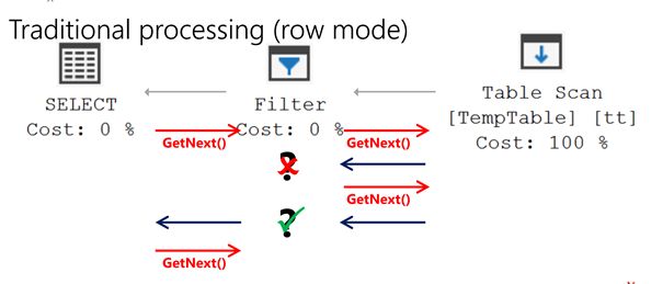
Filter: Dear Table Scan, could I please have a row?
Table Scan: Sure Filter, there you go.
Filter: Thank you. Could I now have another row please?
Table Scan: Sure, have another row.

That seems quite tedious right? Asking for one row over and over. However it is not that bad as that’s exactly the behaviour SQL Server had to offer before version 2014.

What happens though is that at the CPU level execution context is changed. That leads to a reload of the Level 1 Instruction Cache (just quoting Hugo) which is an expensive operation at the CPU level.

So with SQL Server 2014, SQL Server introduced batch mode. Batch Mode means that a handful of rows is transferred between the operators in one go making overall processing more effective.

 

So the dialogue here could go like this (again transcribed from Hugo 🙂 ) :

Filter: Dear Table Scan, could I please have a couple of rows?
Table Scan: Sure Filter, there you go with 600 rows. Have fun.
Filter: Thank you. I’m already done.

Here the Table Scan returns a vector of rows. According to Hugo, the batch size depends on the table and your hardware and is typically something between 600 and 1.000 rows. The filter operation than goes through that vector and marks the relevant rows (imagine a column such as isRelevant with the boolean value true or false).

Batch mode can significantly speed up your query if you have the right workload. Right workload, what does that mean? Typically this makes most sense for analytical queries and aggregation or window functions used. This is exactly the reason why the feature was introduced for ColumnStore, which is a big enabler for analytical queries in a data-warehouse-context. According to Hugo, in a classic transactional system (aka OLTP) batch mode however could slow things down. Think of just a few rows being processed but the additional overhead by batch mode for example.

So yeah just because we couldn’t have batch mode in rowstore queries by default before SQL Server 2019 that didn’t mean that we couldn’t force SQL Server into using batch mode: You could do different kind of tricks to achieve batch mode being used. Read more about it in a blog post (even with a video) by the great Kendra Little. However performing such a hack has some shortcomings:

• It could just break with the next CU or release because you are taking advantage of an undocumented feature.
• There is no intelligence integrated about when to use batch mode or not so you are completely responsible to judge that right and perform repeated performance tests from time to time.

Thus Microsoft realized over the years that people do indeed want Batch Mode on rowstore indexes as well (you could have analytical workloads there too ;-)) and baked Batch Mode for Rowstore in as a true feature. The cool thing is that now the SQL Server optimizer determines whether a query would benefit from batch mode or not. How is that done?
According to Hugo’s presentation the following prerequisites must be met:

• The query uses an “interesting table”: this means a table which has more than 131,701 rows (as of CTP 2.2)
• The query uses interesting operations: this means joins, aggregations or window aggregates with more than 131,701 rows
• The relevant operation does not access any LOB data, XML, spatial datatype, full-text-search or cursors (Hey…who’s doing that anyway? Relax…I am just joking, the app I mainly work with is full of XML :-))

Again go ahead and read more about batch mode on rowstore from the gurus themselves:

• Batch Mode For Row Store: What Does It Help With? (Brent Ozar)
• Batch Mode on Rowstore in Basics (Niko Neugebauer)

Scalar UDF Inlining

It was fun watching Hugo at the session making some jokes on Microsoft’s account about query tuning. However this feature he admitted (and I join him whole-heartedly) truly rectifies the title “Intelligent Query Processing” in contrast to “Adaptive Query Processing”.

Scalar Functions are typically all over the place. Most of us were told not to use them for years however the elegance of encapsulating code within a scalar function has led to the widespread adoption. And you know…once something is out and in the wild it is quite complicated putting the genie back in the bottle.

So if you are reading this blog and have no idea what I am writing about here take a look at this article from over a decade ago at the Database Journal. It also describes some common alternatives to Scalar Functions such as creating a Single-Statement-Inline-Table-Valued-Function….gosh it’s getting late again and I am throwing around jargon here ;-). I have once written a complex function for calculating duration in working hours based on two timestamps and a work calendar in such a function (rather than a scalar one). It did boost performance but ended up in a long select which definitely needed some comments here and there explaining what is done in the code. Long story short…the advice from the article is still relevant…unless you might run SQL 2019 and get a bit more relaxed about that.

Scalar UDF Inlining (codename Froid) is doing some cool magic…the procedural T-SQL code of the scalar function gets converted into equivalent query expressions at compile time. However this rocket-science-technique still is not available to every scalar function out in the wild. Take a look at the DMV sys.sql_modules

SELECT
  OBJECT_NAME(object_id) AS moduleName,
  [definition],
  is_inlineable, /* 1 = function can use inlining */
  inline_type /* 1= inlining is actually turned on for function */
FROM 
  sys.sql_modules
WHERE 
  is_inlineable = 1

It appears that there is just one function (DetermineCustomerAccess) in the sample WideWorldImporters database which is actually inlineable :-).

Go ahead and read more about this from the pros:

• The Coming Froidpocalypse (Erik Darling): A good intro IMHO
• The official documentation on MSDN
• Froid vs Freud: Scalar T-SQL UDF Inlining (Niko Neugebauer)

Approximate Count Distinct

This is a new way of getting a count of distinct values of a table which is a fast but could be imprecise. According to Hugo the Error margin is “within 2% for at least 97% of all use cases” or you get a “3% chance to be more than 2% wrong”…and there’s no limit on how much off you could be in this 3% of all cases.

To be honest I have not found a use case for that function in my environment yet.

But check it out for yourself and read more here:

•  There is a New COUNT in Town (Greg Larsen)
• Approximate Distinct Count (Niko Neugebauer)

Final Thoughts

So wow I am done. I have really struggled with this blog post about Hugo’s session. Why? Because it’s pretty clear to me that I am by no way an expert with this new features. I haven’t seen any of the SQL 2017 features because of running Standard Edition respectively not having an adequate workload or ColumnStore I guess. However SQL 2019 is a game changer bringing a broader variety of those features and so I start learning about it now. For myself it has proven extremely valuable to write that wrap-up of Hugo’s session in my own words. If I put things the wrong way I am grateful for a small hint. Maybe the write-up is valuable to some of you learning about these features as well. I wrote about things in my own words however most of this parts content comes directly from Hugo’s session, Microsoft or other bloggers. If you sense any plagiarism in my writing please let me know and I’d be more than happy to apologize and correct it.